What is Synthetic New Relic?:
New Relic Synthetics is a set of automated scriptable tools to monitor the websites, critical business transactions and API endpoints. A detailed individual results from each monitor run can also be viewed. With access to New relic Insights, in-depth queries of data can be run from Synthetics monitors. Creation of custom dashboards are also possible.
Features of Synthetic New Relic:
- Easy to set up real time instrumentation and analytics
- REST API functions
- Real browsers
- Comparative charting with Browser
- New Relic Insights support
- Advanced scripted monitoring
- Global test coverage
Different types of Synthetic Monitor:
There are four types of monitor.
a) Ping monitor:
Ping monitors are the simplest type of monitor. These monitors are used to check if an application is online. The Synthetics ping monitor uses a simple Java HTTP client to make requests to your site.
b) API tests:
API tests are used to monitor API endpoints. This can ensure that the app server works in addition to the corresponding website. New Relic uses the “http request module” internally to make HTTP calls to API endpoint and validate the results.
c) Browser:
Simple browser monitors essentially are simple, pre-built scripted browser monitors. These monitors make a request to the site using an instance of Google Chrome.
d) Script_Browser:
Scripted browser monitors are used for more sophisticated, customized monitoring. A custom script can be created to navigate to the website, take specific actions and ensure that the specific resources are present.
Creation of Synthetic Monitor:
API Test Monitor:
Step 1:
- Login to new relic monitor
Step 2 – Create synthetic monitor
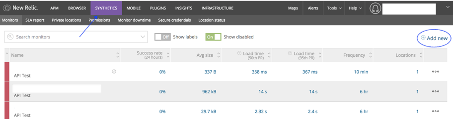
- Click “synthetic” in new relic dashboard after click on the “Add new” in the right up corner.

Step 3: Enter the Required Details
- Select on “API Test” in monitor type.
- Enter the monitor name under details
- Select one location for the monitor under monitoring locations.
- Set the Schedule – Set frequency for monitoring. For example On selecting frequency as 10 mins, The monitor would run this monitor and check for every 10 mins.
- Set Notification – Notification to email ids can be set with help of new alert policy or can be appended to existing alert policy. In case of existing alert policy, Click on “Add to an existing alert policy” and the existing policy can be selected. In case of new policy, email address and policy name has to be given. There are three type of policy,
- By Policy – Only one open incident at a time for this alert policy.
- By Condition – Only one open incident at a time per alert condition
- By condition and entity – open an incident every time a condition is violated.
- Only on completing the above steps, Script can be written by clicking on “Write Your script”
- Click on “create monitor” after the monitor creation steps done.
PING Monitor:
Step 1:
- Login to new relic monitor
Step 2 – Create synthetic monitor
- Click “synthetic” in new relic dashboard after click on the “Add new” in the right up corner.
Step 3: Enter the Required Details
- Select on “API Test” in monitor type
- Enter the monitor name under details
- Enter the URL and enter the response corresponding URL
- Select one location for the monitor under monitoring locations.
- Set the Schedule – Set frequency for monitoring. For example On selecting frequency as 10 mins, The monitor would run this monitor and check for every 10 mins.
- Set Notification – Notification to email ids can be set with help of new alert policy or can be appended to existing alert policy. In case of existing alert policy, Click on “Add to an existing alert policy” and the existing policy can be selected. In case of new policy, email address and policy name has to be given. There are three type of policy,
- By Policy – Only one open incident at a time for this alert policy.
- By Condition – Only one open incident at a time per alert condition.
- By condition and entity – open an incident every time a condition is violated.
- Only on completing the above steps, Ping monitor gets created when clicking on “ Create Monitor”
Synthetic Monitor Functionality:
API Test:
Pass Scenario:
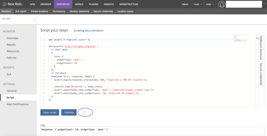
Below script is used to store the data using Post method, then pass the value to the call back function .Call back function is nothing but it is a function is passed into another function as an argument.
Here, call back function has three arguments like error, response and body.
In the below script, comparing the value “gear” and “10” with JSON body value. Both the values are same. Hence no assertion error is triggered.
In case of value mismatch, an assertion error is thrown.
Failure scenario:
In the below script, the values do not match with the JSON body value. Hence an assertion error is thrown.
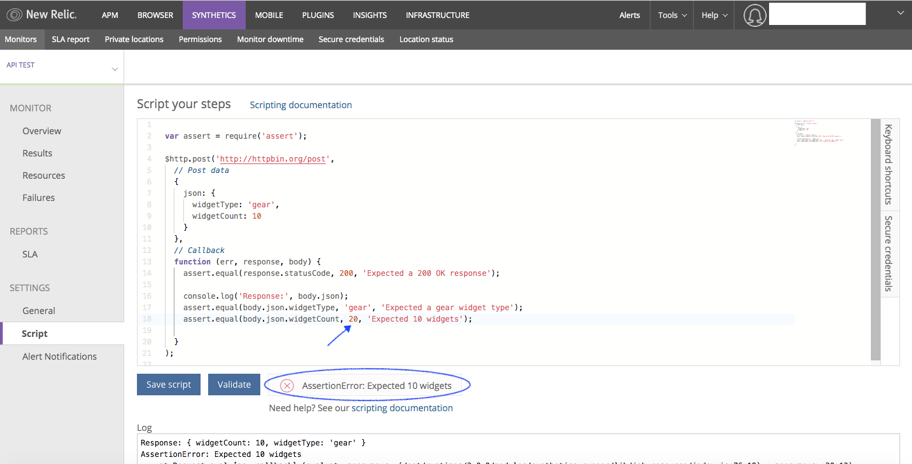
In case of assertion error, an alert will be sent to the mail id given in the notification channel. The Assertion error will not be resolved until the Value is made “10”.
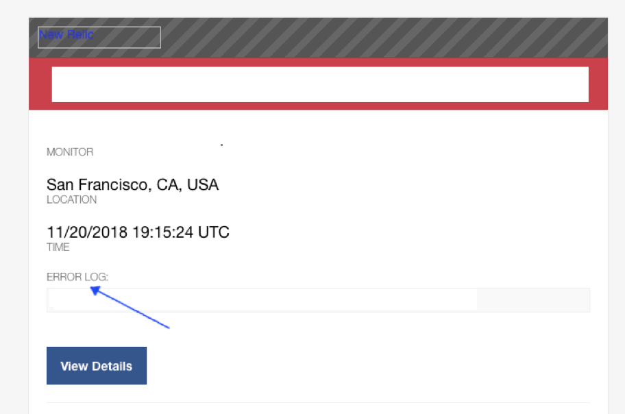
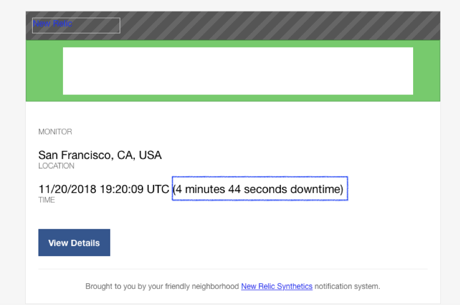
Mail Alert: (Ping & API Test)
The error log can be seen as below:
After the error is fixed, an update would be sent to the notification channel
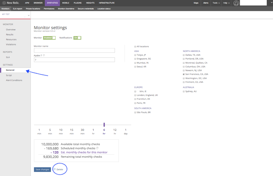
Delete a Monitor: (Ping & API Test)
- From the Monitors list, select the monitor which needs to delete.
- In the selected monitor, under settings click on General to view the monitor settings page.
- Select the trash icon, it will show alert popup and click on “ok” in alert popup then monitor will delete.